Sizing a generative AI deployment looks like a procurement question and behaves like a search problem. What goes in is a model, a service level objective and a budget. What has to come out is a chip, a count of that chip, a serving engine, a parallelism split, a quantization scheme and a batching policy — six answers that are only correct together. Between the question and the answer sits a space no team can walk by hand. The engine we built to walk it is Bud Simulator, and we have open-sourced it — the code is at BudEcosystem/simulator on GitHub.
It ships as the sizing engine in Bud AI Foundry's control plane — the part of Layer 04 that decides what a deployment should look like before anything is placed on a cluster — and a memory-and-speed variant of the same engine runs in Bud Gaia's discovery layer, on a laptop, deciding which model is worth downloading. This piece is about how it works: what it is asked, how it predicts a number it has never measured, how it searches, and how far you should trust the answer.
The question nobody can brute-force
Start with what is actually being chosen. A serving deployment is not one decision; it is a product of decisions, and each one multiplies the space rather than adding to it.
| Decision axis | What it sets | What it trades against |
|---|---|---|
| Accelerator and count | Peak compute, memory capacity, memory bandwidth, interconnect. | Capital or rental cost, and power. |
| Serving engine | Which kernels, scheduler and cache implementation run underneath. | Model and modality coverage. |
| Tensor and pipeline split | How the model is cut across devices. | Collective traffic against per-device memory pressure. |
| Quantization and dtype | Weight and activation footprint, and the bytes moved per token. | Accuracy, and kernel availability on that chip. |
| Batching and scheduler policy | How many requests share a forward pass. | Time-to-first-token against throughput. |
| KV cache and block size | How many concurrent sequences fit in memory. | Maximum context against maximum concurrency. |
Table 1 — the six axes a serving configuration has to fix. None of them can be set correctly in isolation, because each one moves the constraint the next one is working against.
Multiply those out and the number gets large very quickly. vLLM alone carries on the order of 400 million configuration permutations for a single-node deployment. That figure is already the interesting part of the problem, and it understates it, because it assumes the hardware is fixed. It is not: the point of a hardware-agnostic platform is that the chip is also a variable, and Bud Simulator carries 72 hardware profiles — NVIDIA, AMD and Intel accelerators, Google TPUs, AWS silicon, specialty ASICs, and Intel, AMD and ARM CPUs. Put the two together and the space to be searched is around 3 × 10¹⁰.
A space that size is not a tuning exercise. At one benchmark run per configuration — thirty minutes of a rented accelerator, call it five dollars — walking even a millionth of it would cost more than the cluster. The reason enterprises staff a GenAI systems engineering team is largely this: somebody has to guess well, because nobody can measure exhaustively.
Why measurement alone does not close the gap
The instinct is to benchmark your way out. It fails for three separate reasons, and it is worth separating them, because each one is answered by a different part of the simulator.
- You cannot benchmark hardware you do not have. The most valuable sizing questions are asked before purchase — should this run on the H200s we are quoted, the MI300Xs we are also quoted, or the L40S fleet already in the rack? A benchmark answers only for the third.
- The optimum moves with the workload, not just the model. The same model serving 8K-token document summaries and 300-token support replies wants different batch sizes, different cache blocks and often different chips. A benchmark result is a point, and you need a surface.
- Per-request latency is not the number you are held to. Production is judged on p99 under a concurrent arrival process with continuous batching and queueing. Measuring one request tells you very little about the ninety-ninth percentile of ten thousand.
The third point deserves emphasis, because it is where most spreadsheet sizing quietly breaks. A model that produces a token every 20ms in isolation does not produce a token every 20ms when 250 sequences are resident and the scheduler is preempting to admit new prefills. The gap between those two numbers is the gap between a sized deployment and a surprised one.
The expensive chip is not always the cheaper answer. Measured on tokens per dollar, the A10G delivers up to 2.6× the value of an A100 for small requests, while for large requests the A100 beats the A10G by 1.5×. The crossover depends on request size, request rate and the SLO — which is exactly why the decision cannot be made from a price list.
Three ways to predict a number you have not measured
Bud Simulator does not use one model of performance. It uses three, stacked by cost and fidelity, because no single one is both cheap enough to score a billion candidates and faithful enough to commit hardware on.
| Tier | What it models | What it misses | Where it runs |
|---|---|---|---|
| Analytical roofline GenZ-derived |
Prefill and decode as closed-form functions of FLOPs, memory capacity, bandwidth and interconnect. | Kernel efficiency, scheduler behaviour, framework overhead. | Every candidate in the space, at effectively zero cost. |
| Learned regressors XGBoost |
The residual between the analytical estimate and what the hardware actually did, fitted to measured runs. | Anything outside the distribution it was trained on. | Shortlisted candidates on hardware with measured history. |
| Event-driven serving simulator | Arrivals, queueing, continuous batching, preemption and cache pressure over time. | Nothing about the physics — it takes its per-step numbers from the two tiers above. | The final handful, where p99 has to be defensible. |
Table 2 — three prediction tiers, each answering what the one above it cannot. The stack is the design: an analytical model alone is fast and wrong at the margins; a simulator alone is faithful and far too slow to search with.
Tier one — the roofline
The analytical tier abstracts every accelerator into four numbers: peak FLOPs, memory capacity, memory bandwidth and interconnect bandwidth. That is enough to place any model on a roofline, and the roofline is enough to explain most of what a generative AI deployment does.
The insight it encodes is that the two phases of inference live in different regimes. Prefill processes the whole prompt at once — large matrix-matrix work, high arithmetic intensity, compute-bound. Decode emits one token per sequence per step, which means reading the entire weight set to produce a single token: matrix-vector work, low arithmetic intensity, bandwidth-bound. They are not two settings of the same dial. They are two different bottlenecks in the same deployment.
The same arithmetic produces the hardest constraint in the whole exercise before it produces any performance number at all: will it fit. Weights plus the KV cache at the target concurrency and context length must sit inside aggregate device memory. That single inequality gives the minimum chip count for a candidate, and it is a yes-or-no gate — a configuration that fails it is not slow, it is impossible. Bud Simulator computes it first and discards on it first, which is what makes the rest of the search affordable.
For configurations that use only tensor and pipeline parallelism, this whole tier reduces to a closed-form calculation with no iteration at all. That path exists precisely so the top of the funnel stays free.
Tier two — the learned residual
A roofline is an upper bound on a good day. Real kernels do not hit peak, schedulers add overhead, and two accelerators with identical spec sheets can differ by tens of percent on the same model. The analytical tier cannot see any of that, because none of it is in the four numbers.
So the second tier learns it. Gradient-boosted regressors, trained on measured latency and throughput across the hardware catalogue, predict what the analytical model will be wrong by — and the simulator exposes both paths explicitly, so an operator can ask for the heuristic answer or the regressor answer and compare them. Where measured history exists, the regressor is the better estimate. Where it does not, the heuristic is the only estimate, and the system says so rather than quietly extrapolating.
That honesty is a named feature. For hardware absent from the measured catalogue — a chip announced but not yet in anyone's rack — predictions come back on a confidence ladder rather than as a flat number, so a sizing decision can be weighted by how much evidence stands behind it.
Tier three — the queue
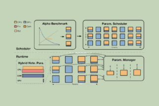
The last tier stops modelling a request and starts modelling a service. An event-driven serving simulator replays a generated workload — arrival distribution, prompt and completion length distributions, concurrency ramp — through the scheduler the candidate would actually run, with continuous batching, preemption and cache eviction in play.
This is the only tier that produces a defensible p99, and it is far too expensive to run on more than a shortlist. On multi-node candidates it also pulls in collective and network simulation, because once a model is split across nodes the all-reduce traffic is frequently the thing that decides between two otherwise identical plans.
Most of what separates a plausible p99 from a real one lives in this tier, and it is worth being specific about what it carries:
- Memory is not one pool. HBM, DRAM, DDR, CXL and NVMe are modelled as tiers with their own spill and fill latencies — which is what lets a candidate that overflows HBM be costed rather than simply rejected.
- The cache is part of the workload. Prefix caching under LRU, LFU or ARC, with shared-prefix detection and hit-rate analysis. A system prompt shared across every request changes the arithmetic, and pretending otherwise flatters the result.
- Prefill and decode can be separated. Disaggregated pools are modelled with M/M/1 queueing, because splitting the two phases onto different hardware is often the plan that wins — and it cannot be evaluated at all without a queueing model.
- Arrivals are a distribution, not a rate. Poisson, bursty and trace-driven patterns, because a workload that averages 200 requests per second but arrives in bursts needs different headroom from one that trickles.
- Speculative decoding is modelled, not assumed. A draft-verify pipeline with an acceptance-rate estimate, so the speed-up is predicted rather than taken from a blog post.
It also produces a number most sizing exercises never reach: power. The simulator carries a physics-based model with a seven-component breakdown — compute, memory, interconnect, cooling, PSU loss, idle draw and leakage. For anyone sizing on-premises capacity, that is not a footnote. It is the difference between a rack that fits the power envelope and one that does not, and it feeds the energy half of cost per token directly.
Searching, not enumerating
Three predictors give you a score for a candidate. They do not give you the candidate. With tens of billions of them and several objectives that genuinely conflict, the search itself has to be a designed component.
Bud Simulator uses a multi-objective genetic search — NSGA-II — over cost, latency and throughput simultaneously. The choice matters. A single-objective optimiser needs you to collapse those three into one number with weights you do not actually know; NSGA-II instead returns the Pareto frontier: every configuration for which you cannot improve one objective without giving up another. Everything off the frontier is dominated — strictly worse on some axis and better on none — and can be discarded without an opinion about priorities.
Ordering matters here in a way that is easy to get wrong. Optimising cost first and checking the SLO afterwards produces cheap configurations that do not work, then a scramble to add hardware. Gating on feasibility first and optimising cost within the survivors produces a plan that is both correct and the cheapest correct one. The second ordering is also what makes the problem tractable, since the gate removes most of the space before the expensive tiers ever run.
The objective is an input, not a result
All of which depends on someone having said what "fast enough" means. This is the step most deployments skip, and skipping it is expensive in a counter-intuitive direction: the default failure is not under-provisioning, it is over-provisioning against a target nobody needed.
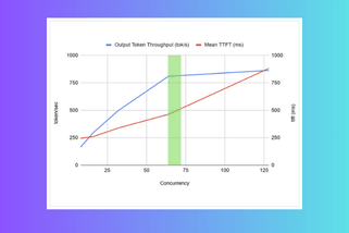
We have written about this before. Generating tokens faster than a person can read them is spend with no return. On an Intel Xeon Platinum 8592V, Llama 3.1 8B delivers 120ms time-to-first-token at 30 concurrent users; letting time-to-first-token rise to 220ms doubles concurrency with no perceptible change in user experience. Two configurations, the same hardware, twice the served population — and the difference is entirely a declared objective.
Every configuration that beats the SLO by a wide margin is a configuration you are paying for twice: once in hardware, and once in the users it could have served and did not.
So the simulator takes the objective as a first-class input rather than deriving it. Its library carries 112 pre-built workload profiles, each with its own SLO shape, because the shape differs far more than the numbers do.
| Workload | What the SLO is actually about | What the sizing follows |
|---|---|---|
| Chat and assistants | Time-to-first-token inside human reaction time; token rate at or slightly above reading speed. | Batch up to the reading-speed floor, then spend the headroom on concurrency. |
| Code completion | Time-to-first-token dominates — a suggestion that arrives late is not used at all. | Smaller batches, prefill-weighted hardware, tighter admission control. |
| Summarisation and batch NLP | No human in the loop. End-to-end job time is the only target. | Maximum batch, maximum concurrency, latency traded away entirely. |
| Agentic and tool-using traffic | Many short model calls per task; per-call overhead compounds across the chain. | Warm capacity and gateway overhead matter more than peak throughput. |
Table 3 — four workload shapes and the sizing each one implies. A single "latency target" number cannot express any of these; the profile is what carries the distinction into the search.
The payoff of getting this right is measured in goodput — useful tokens delivered inside the objective, rather than tokens per second in the abstract.
Bring a model, a workload and the hardware you own or are being quoted. We will run the sizing against your SLO and show the frontier.
From verdict to deployment
A sizing tool that produces a PDF has done a third of the job. The reason Bud Simulator sits inside the control plane rather than beside it is that its output is the deployment — the configuration it returns is the configuration Bud Runtime applies. That is what "zero-config" means in practice: not that there are no settings, but that nobody types them.
What you hand it is small. The whole point of the workload library is that the request describes an outcome rather than a configuration.
usecase: customer-support-chat   # one of 112 profiles
model:   llama-3.1-8b-instruct
slo:
  ttft_p99_ms: 400
  tpot_p99_ms: 50              # ~20 tok/s — above reading speed
  concurrency: 250
hardware: [owned, catalog]     # what you have + what you could buy
optimise: cost_per_million_tokens
Illustrative — the shape of the question, not a literal API contract. The simulator exposes the real thing as a REST service over models, hardware, use cases and simulations, with a wizard in front of it for people who would rather not write the file.
Because the same engine runs before and after deployment, the sizing is not a one-time artefact. When traffic shifts, a model is replaced, or a new accelerator enters the fleet, the question is re-asked against the observed workload rather than the assumed one — which is the difference between a cluster that was right in March and a cluster that is right now.
The other half: training
Everything so far has been about serving. The same engine answers the mirror-image question for training, where the constraint is harsher: inference that does not fit degrades, but training that does not fit does not start.
The memory model is the part worth dwelling on, because the naïve version is wrong in a specific way. Weights, gradients, optimizer state and activations do not all peak at the same moment — forward, backward and optimizer phases are tracked separately and the total is the maximum of the phase peaks, not the sum of the parts. Get that wrong and you either buy hardware you do not need or discover at step one that you cannot run.
| Stage | Method | Weights | Gradients | Optimizer | Activations | Total / GPU |
|---|---|---|---|---|---|---|
| SFT | Full | 17.7 | 35.3 | 70.7 | 10.9 | 148.0 |
| SFT | LoRA | 17.7 | 0.1 | 0.3 | 10.9 | 31.9 |
| SFT | QLoRA | 4.4 | 0.1 | 0.3 | 10.9 | 17.3 |
| DPO | LoRA | 17.7 | 0.1 | 0.3 | 10.9 | 51.3 |
| PPO | Full | 17.7 | 35.3 | 70.7 | 10.9 | 323.0 |
Table 4 — predicted training memory in GB per GPU for Llama 3.1 8B at batch 4, sequence 2,048, from the simulator's own sample output. DPO and PPO totals include the reference and reward models they carry alongside the policy, which is why PPO lands at 323 GB while full SFT on the same model needs 148 GB. The spread between full SFT and QLoRA — 148 GB against 17.3 GB — is the difference between a multi-node job and a single card.
Around that sit the combinations a training platform actually has to support: 14 training stages (SFT, DPO, PPO, GRPO, KTO, ORPO, SimPO, IPO, RM, RLOO, REINFORCE, CPO, PT and a detailed PPO variant), six fine-tuning methods (full, LoRA, QLoRA, DoRA, PiSSA and freeze) with accurate parameter counting, and 30-plus optimizers from AdamW and Lion through Adafactor, GaLore, LOMO, Muon, schedule-free and 8-bit variants — each with its own optimizer-state cost, which is exactly the term that dominates the table above.
Distribution is modelled too: tensor, pipeline, data and expert parallelism, ZeRO stages 0 through 3, pipeline 1F1B bubble modelling, sequence parallelism splitting activation memory across the tensor-parallel group, and selective or full gradient checkpointing. The outputs are the ones a team can act on — end-to-end time, cost and model FLOPs utilisation against a dataset token count; a ranking of candidate GPU clusters by throughput, ETA, cost or a composite score; and generated configuration files, in LlamaFactory YAML, DeepSpeed JSON and Accelerate form, with launch commands.
The serving question is "how much hardware do I need to hold this SLO." The training question is "which cluster finishes this run soonest, or cheapest, and can it run at all." Both are answered by the same memory and roofline machinery — which is why the sizing case for a GPU purchase does not have to be assembled twice from two different tools.
When the accelerator is a CPU
Bud's platform argument leans on CPUs doing real inference work, and a sizing engine that models GPUs precisely and CPUs vaguely would quietly undermine it. So the CPU path is not a fallback with a fudge factor — it is its own operator framework.
What it models is the set of things that actually determine CPU inference throughput: instruction set — AMX, AVX-512, AVX2, SVE and NEON, each with its own throughput multiplier; the cache hierarchy, L1 through L3, with bandwidth estimation and KV-cache placement; NUMA topology across sockets and CCDs, with cross-node traffic estimated rather than ignored; the threading model, physical cores against SMT, with NUMA-pinned execution; and frequency scaling under thermal and power limits. GEMM, attention and reduction operators each get a CPU-specific roofline.
| CPU | Throughput, batch 1 | TTFT, batch 1 | Throughput, batch 32 | TTFT, batch 32 |
|---|---|---|---|---|
| AMD Turin (Zen 5) | 42.7 tok/s | 100 ms | 1,178 tok/s | 3,212 ms |
| Intel Granite Rapids | 35.6 tok/s | 114 ms | 982 tok/s | 3,660 ms |
| NVIDIA Grace (ARM) | 35.6 tok/s | 133 ms | 912 tok/s | 4,253 ms |
| AWS Graviton4 (ARM) | 32.0 tok/s | 246 ms | 520 tok/s | 7,868 ms |
Table 5 — predicted CPU inference for Llama 3.1 8B at BF16, from the simulator's BudEvolve analysis. Note what batching does here: throughput rises roughly 28× from batch 1 to batch 32 on Turin, while time-to-first-token rises 32×. That is the same trade the roofline predicts for GPUs, on silicon most sizing tools decline to model at all.
The hardware catalogue reflects the same intent. Its 72 profiles span NVIDIA from V100 through GB200, AMD Instinct, Google TPU v4 to v6, Intel Gaudi 3 and Max, AWS Trainium and Inferentia, specialty silicon from Cerebras, Groq and SambaNova — and, in the same catalogue rather than a separate one, Intel Xeon, AMD EPYC and ARM server CPUs.
BudEvolve: running the search backwards
Everything described so far takes hardware as given and searches for a configuration. BudEvolve is the part that inverts the question — and it is the piece most likely to matter to anyone specifying infrastructure rather than deploying on it.
- Hardware design-space exploration. Sweep FLOPS, bandwidth, memory capacity and interconnect as free variables and find which combination the workload actually wants. The output is a specification, not a purchase order — useful when the question is "what should we ask vendors for" rather than "which of these three quotes".
- Parameter sensitivity, ranked. Morris-method analysis over configuration and hardware parameters, ordered by their effect on throughput and latency. It answers the question behind most tuning work: which knob is worth touching at all.
- What-if sweeps. Single-parameter curves, so the shape of a dependency is visible rather than inferred from two measured points.
- Algorithm evolution. The unusual one: using an LLM to mutate and evolve the scheduling and cache-eviction algorithms themselves — batch scheduling, KV-cache eviction policy, and CPU-optimised schedulers that are NUMA-aware, L3-budget-aware and TTFT-aware.
That last item is worth separating from the rest. The first three are analysis on top of the simulator. The fourth uses the simulator as a fitness function — which is what a fast, calibrated performance model lets you do once you have one, and a reason to care about simulation accuracy beyond the sizing report it was built for.
Where the answer changes the bill
The commercial case for simulation is not that it saves engineering time, although it does. It is that the cost-optimal answer is usually not the one a human would pick, because humans pick one chip and standardise on it.
Once cost per token is the objective and the hardware catalogue is a variable, the search routinely returns mixed answers: commodity GPUs for small requests, high-end accelerators for large ones, CPUs for the parts of the pipeline that never needed an accelerator. That is the basis of heterogeneous serving, where splitting a workload across hardware tiers has produced cost savings of up to 77% against a uniform high-end fleet. The simulator is what makes the split decidable rather than a hunch — a heterogeneous plan has more moving parts than a homogeneous one, and there is no point proposing it if you cannot predict what it will do.
Bud AI Foundry's headline TCO claim rests directly on this. It is worth stating with its baseline attached rather than as a number.
| Claim | Metric | Comparison baseline | Conditions |
|---|---|---|---|
| ~3× performance | tokens per second | Naïve serving, same GPU | Batch and precision targets held constant |
| 12× cold start | time to first token from zero | Standard container start | Scale-from-zero, same model and accelerator |
| Under 1ms gateway | added p99 latency | Inference time isolated | Measured at 10K+ QPS |
| 6× better TCO | fully-loaded $ per million tokens | GPU-only single tier | Hybrid workload sized by Bud Simulator, equal SLA |
Table 6 — Bud AI Foundry's performance claims with their baselines. The last row is the simulator's: the comparison is a hybrid deployment it sized against a single-tier GPU deployment holding the same SLA, with hardware, power and idle reclamation included in the cost.
The same engine, on a laptop
The enterprise version of this question is which cluster to buy. The personal version is which model to download, and it has the same structure with much harder constraints — one device, no elasticity, and a user who is also using the machine for something else.
In Bud Gaia, the personal AI operating system, Bud Simulator sits in the discovery layer next to Model Finder. An application asks for an outcome rather than a filename — good at sales conversations, speaks Malayalam, answers in about a second. Model Finder shortlists open models that can do the job on skill benchmarks, language and licence. Bud Simulator then predicts memory and speed for each candidate on that exact chip, beside everything already resident, before a byte is downloaded.
| Candidate | Good at the job? | Fits the machine? | Around a second? |
|---|---|---|---|
| A 13B generalist | Decent | No — 26.8 GB, will not fit | Not reached |
| A 3B chat model | Weak on sales | Yes — 6.1 GB | Yes — about 0.3 s |
| A 7B sales-tuned model | Best in class | Yes — 14.2 GB | Yes — about 0.6 s |
Table 7 — an illustrative shortlist and the simulator's verdict, as shown on the Bud Gaia page. Today this is a week of guesswork and several 20-gigabyte downloads. The fit check is what turns it into a decision.
How wrong is it, and how would you know?
A prediction that cannot be audited is a guess with better typography. The most useful thing a simulator can publish is therefore its own error bars, so here they are.
| Quantity | Stated accuracy | Why it sits where it does |
|---|---|---|
| Memory | ±10% | Closest to arithmetic — weights, cache and activations are counted, not estimated. |
| Throughput | ±15% | Depends on kernel quality and scheduler behaviour, which a roofline cannot fully see. |
| Training time | ±20% | Compounds every other error over hours of wall clock. |
Table 8 — the published accuracy bands. The ordering is the informative part, and a sizing decision should be read against it: a 4% predicted cost gap between two candidates is noise, a 3× gap is not.
Four things hold those numbers up, and it is worth being plain about the limits of each.
- No magic numbers. Every efficiency constant — model and memory-bandwidth utilisation bands, CPU STREAM efficiency, optimizer-state bytes, per-device TDP — is sourced from a datasheet, an ISA specification, a published benchmark or a measured microbenchmark, rather than fitted until the answer looked right. Physical-limit invariants hold across every simulatable device: utilisation never exceeds one.
- Validated against public baselines. MLPerf Training, DeepSpeed ZeRO, Megatron-LM and vendor specifications — targets someone else published, which is the only kind worth validating against.
- Tested as software, not just as a model. 900+ tests across 60+ files, covering inference, training, serving, the CPU path, BudEvolve and the API. A performance model is a large body of arithmetic; most of the ways it goes wrong are ordinary bugs.
- Two methods, visible side by side. The heuristic and regressor paths are separately addressable. When they disagree materially on a candidate, that disagreement is itself the signal — it usually means the configuration sits outside the region the regressor has seen. For accelerators with no measured history at all, the answer comes back on a confidence ladder rather than dressed up as an equal-standing estimate.
This is a prior, not a measurement. It narrows a space of 3 × 10¹⁰ to a handful of candidates worth putting real traffic through, and it is reliably right about which region of the space to be in. It is not a substitute for running your workload on the shortlist before you sign a purchase order — and the fastest way to find out where it is wrong for you is to do exactly that, then feed the result back in.
That last point is the design philosophy rather than a caveat. The simulator is a component in a loop that also contains a gateway collecting real latency, a metrics plane rolling it up, and a scheduler that can re-place a deployment. Each production request is evidence about the next sizing decision. A sizing tool that sat outside that loop would be stuck with whatever it assumed on day one.
Related white paper The Enterprise Buyer's Guide to Foundational AI Platforms The responsibility ledger, the full capability inventory, and where simulation sits across twelve platforms →- Serving configuration is a search problem of roughly 3 × 10¹⁰ candidates, not a tuning exercise.
- Three stacked predictors make it tractable — a closed-form roofline, learned regressors, then a serving simulator on the finalists.
- Feasibility is gated before cost is optimised, and the SLO is a declared input rather than a result.
Sources and scope. The 400-million-permutation figure for a single-node vLLM deployment is as stated in Bud's CSP transformation white paper. The 72 hardware profiles, the ±10% / ±15% / ±20% accuracy bands, the 900+ tests, the validation baselines (MLPerf Training, DeepSpeed ZeRO, Megatron-LM, vendor specifications), the 14 training stages, six fine-tuning methods and 30-plus optimizers, the CPU and BudEvolve capabilities, and the sample results in Tables 4 and 5 are from the BudEcosystem/simulator repository. The 112-workload profile library and the simulator's REST surface are from the capability inventory in The Enterprise Buyer's Guide to Foundational AI Platforms; the learned-regressor prediction path is a platform capability from the same inventory rather than part of the open-source engine, which is analytically calibrated. Goodput gains (2.0–3.14×, 3.2×, 4.48×), the SLO-precision figures and the Intel Xeon Platinum 8592V time-to-first-token and concurrency numbers are from our deployment-templates testing, reported in full in the SLO-driven optimisation post. Tokens-per-dollar comparisons between the A10G and A100, and the up-to-77% heterogeneous-serving saving, are from the heterogeneous hardware post and the research it reviews. Bud AI Foundry's 3× / 12× / under-1ms / 6× claims carry the baselines shown in Table 4. Figures 1, 2 and 3 and the shortlist in Table 5 are schematic: the decomposition in Figure 1, the relative units in Figure 2, and the cost and latency values in Figure 3 and Table 5 are drawn to show shape and are not measured results. Substitute your own workload distribution, hardware quotes and SLO for a firm number.